Responsible	Samuel Schoenenberger
Last Updated	10/12/2025, 12:48:54 PM
Last Author	Kai Berszin

Actuator Controllers

Scope

The chapters in this section describe how the actuator controllers work. Includes mathematical description as well as description of MATLAB implementation of:

1. Torque to actuator mapping
2. Reaction wheel desaturation controller

Satellite Torque to Actuator Command Mapping

The pointing and science controllers return the desired torque on the satellite in the satellite frame. To produce this torque, we need to find which commands to send to the reaction wheels and magnetorquers.

Reaction wheel command mapping

Mathematical explanation

The goal of the reaction wheel command mapping is to decompose the torque we want to produce into the torques created by each reaction wheel. This is done by solving the following quadratic program:

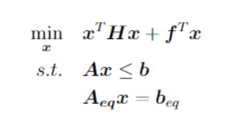
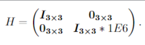
where $\vec{H}$ is the Hessian matrix and $\vec{f}$ is the gradient of the cost function. The optimization variables $\vec{x}$ consist of the torques of each reaction wheel and the torque error (i.e., the discrepancy between the torque exerted by the reaction wheels mapped in the satellite coordinate system and the requested torque). Thus, $\vec{x}$ is defined as follows: $\vec{x} = (\tau_1, \tau_2, \tau_3, T_{err,1}, T_{err,2}, T_{err,3})^T.$ We want to minimize the sum of the square of $\vec{\tau}$ and $\vec{T_{err}}$, each with their individual weights $\vec{Q_\tau}$ and $\vec{Q_T}$. This cost function can be written as $J(\vec{\tau}, \vec{T_{err}}) = \vec{\tau}^T \vec{Q_\tau} \vec{\tau} + \vec{T_{err}}^T \vec{Q_T} \vec{T_{err}}.$ Thus, the hessian matrix $\vec{H}$ is a diagonal matrix with $\vec{Q_\tau}$ and $\vec{Q_T}$ and the gradient $\vec{f} = \vec{0}$. The main objective is to minimize the torque error, therefore its penalty weight $\vec{Q_T} = 1E6$ is chosen to be significantly larger than the penalty for the individual torques $\vec{Q_{\tau}} = 1$. Thus, $\vec{H}$ can be written as

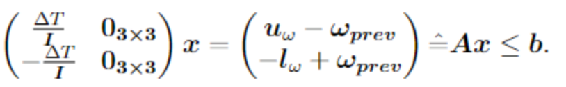
The inequality constraints are used to limit the maximum speed of the reaction wheels. The speed of a reaction wheel after applying the torque $\tau$ can be written as a first order explicit Euler integration $\omega = \omega_{prev} + \Delta T\frac{\tau}{I}$ where $\omega_{prev}$ is the rotation speed of the reaction wheel before applying the torque (i.e., when this function is entered), $\omega$ is the speed after $\tau$ was applied. $\Delta T$ is the period of the control cycle and $I$ is the moment of inertia of the wheel. The rotation speed has an upper bound $u_\omega$ and a lower bound $l_\omega$: $l_\omega \leq \omega \leq u_\omega \Leftrightarrow l_\omega \leq \omega_{prev} + \Delta T\frac{\tau}{I} \leq u_\omega.$ This can be reformulated into $\frac{\Delta T}{I} \tau \leq u_\omega - \omega_{prev}$ $-\frac{\Delta T}{I} \tau \leq - l_\omega + \omega_{prev}$ which can easily be formulated into the matrix-vector from $\vec{A} \vec{x} \leq \vec{b}$

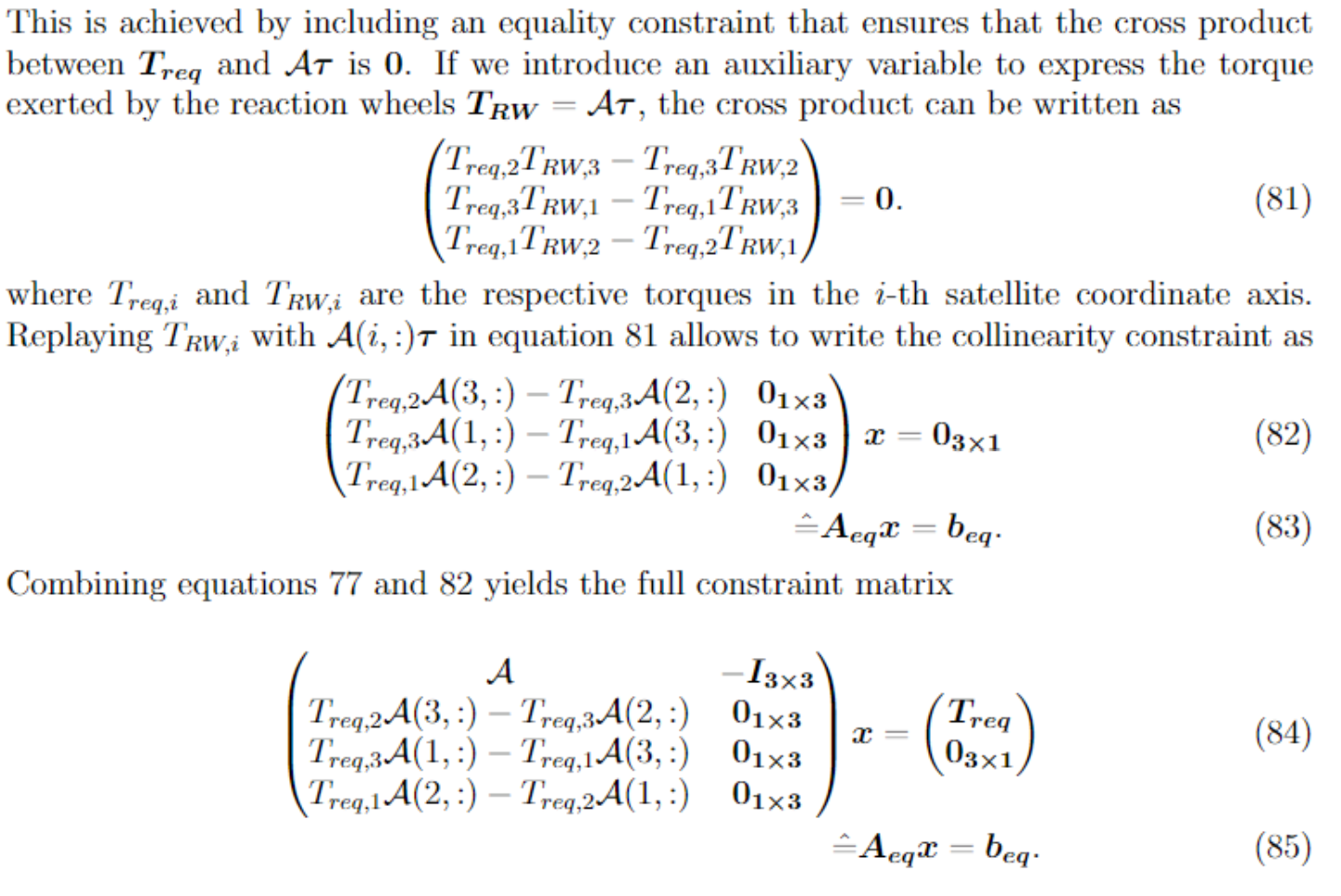
The equality constraints $\vec{A_{eq}} \vec{x} = \vec{b_{eq}}$ are used to define two relationships: First, the relationship between $\vec{T_{err}}$ and $\vec{\tau}$ and second, a collinearity constraint which enforces that the resulting torque vector is collinear to the requested torque vector.

First, let's define $\mathcal{A}$ which is the matrix containing the rotation axis of the reaction wheels $\mathcal{A} = [\vec{a_1}, \vec{a_2}, \vec{a_3}] \in \mathcal{R}^{3\times3}$ where $\vec{a_i}$ is the rotation axis of the $i$-th reaction wheel. Therefore, the torque of the $i$-th reaction wheel can be mapped in the satellite coordinate system via $\vec{T_i} = \vec{a_i} \tau_i$. We'll use this relationship to express the torque error $\vec{T_{err}}$ (i.e., the difference between the torque from the reaction wheels and the requested torque) in the satellite coordinate system via $\vec{T_{err}} = \mathcal{A} \vec{\tau} - \vec{T_{req}}$ where $\vec{T_{req}}$ is the requested torque (ideally, the torque exerted by the reaction wheels should equal the requested torque). This equation can be rewritten as $\mathcal{A} \vec{\tau} - \vec{T_{err}} = \vec{T_{req}}$ $\hat{=} (\mathcal{A} , -\vec{I_{3\times3}}) \vec{x} = \vec{T_{req}}$ $\hat{=} \vec{A_{eq}} \vec{x} = \vec{b_{eq}}$ The torque collinenarity is achieved if and only if the cross product between the torque produced by the reaction wheels and the requested torque is 0 $cross (\mathcal{A} \vec{\tau}, \vec{T_{req}}) = \vec{0}.$

The optimization problem can be solved by any solver for quadratic programs (QPs).

Reaction wheel input calculations

By solving the optimization problem from the previous subsection, we obtain the torque $\tau_i$ to be applied by the i-th reaction wheel. However the reaction wheels use the target rotational velocity as their inputs.

If a reaction wheel with moment of inertia $I$ around its rotation axis is spinning with rotational velocity $\omega_{prev}$ when entering the actuator mapping function, we apply torque $\tau$ and the discretization step length is $\Delta T$, the rotational velocity after the torque was applied will be $\vec{\omega} = \vec{\omega_{prev}} + \frac{\vec{\tau}}{\vec{I}}\Delta T.$ We use $\vec{\omega}$ as the input to the reaction wheel.

Feasibility Analysis

The optimization problem to calculate the reaction wheel torques is designed to always be feasible, meaning that there always exists an $\vec{x}$ so that the constraints in the optimization problem can always be fulfilled by $\vec{x} = \vec{0}$. This is achieved by the torque error being included in the cost function rather than a constraint. Considerations must be made in the event of a malfunction of one reaction wheel. In that case, that reaction wheel is disabled and the corresponding axis in $\mathcal{A}$ is set to $\vec{0}$. As long as the remaining axes matrix $\mathcal{A}$ has column rank 3, i.e., the columns of $\mathcal{A}$ span a 3-dimensional space, the satellite can be controlled (even though the maximum exerted torque is reduced due to the missing reaction wheel).

The only condition under which the optimization problem can become infeasible is if the current reaction wheel speed $\vec{\omega_{prev}}$ exceeds the speed boundary defined in in the inequality constraint due to measurement errors. If no $\vec{\tau}$ can be calculated without exceeding the torque boundary for the reaction wheels, the problem becomes infeasible. This can be alleviated by limiting $\vec{\omega_{prev}}$ before entering the torque mapping function.

Implementation

The implementation can be tested in run_files/combinedActuatorMapping/run_testCombinedActuatorControl.m. The optimization problem can be solved by any solver for quadratic programs (QPs). Currently MATLAB's quadprog() is used. This is implemented in ctrl/actuator_control/torqueTo3RWsMap.m.

Magnetorquer command mapping

Mathematical Description

Magnetorquers create a torque on the satellite by creating a magnetic field that interacts with Earth's magnetic field. Since the resulting torque is perpendicular to Earth's magnetic field, the magnetorquers can only create a torque in 2D.

A quadratic program is defined that calculates the optimal magnetorquer voltages from the desired torque in satellite frame. The decision variable $\vec{x}$ can be written as $\vec{x} = (U_1 , U_2 , U_3 , T_{res, x} , T_{res, y} , T_{res, z} , |T_{res, x}| , |T_{res, y}| , |T_{res, z}| )^T$ where $U_i$ is the voltage of the $i$-th magnetorquer, $T_{res, k}$ is the residual torque around the $k$-th satellite axis and $|T_{res, k}|$ is the absolute value of the latter. The residual torque is the disrepancy between the requested torque and the torque that can be delivered by the magnetorquers.

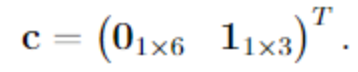
The torque created by the $i$-th magnetorquer can be written as $\vec{\tau_{MT, i}} = \frac{o \vec{a_{MT, i}} \times \vec{B_{sat}}}{R_i} U_i$ Thus, the residual torque vector is defined as $\vec{T_{res}} = \vec{T_{req}} - \sum_{i=1}^3 \vec{\tau_{MT, i}}$ The absolute torque residual $|T_{res, k}|$ is defined as $|T_{res, k}| \geq T_{res, k}$ $|T_{res, k}| \geq -T_{res, k}$ The objective is to minimize the sum of absolute residual torques $\sum_{k=\{x,y,z\}} |T_{res, k}|$ which translates into the cost vector

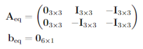
The optimization problem is defined via matrices and vectors. The equality constraints are encoded in the $\vec{A}$ and $\vec{b}$ and the inequality constraints via $\vec{A_{eq}}$ and $\vec{b_{eq}}$. The equality constraints are defined as follows:

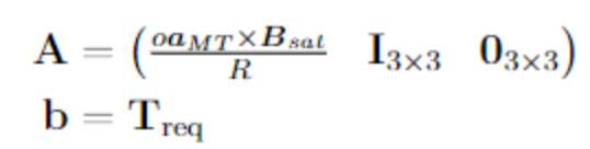
Similarly, the inequality constraints are encoded in $\vec{A_{eq}}$ and $\vec{b_{eq}}$ as follows:

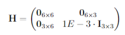
With the upper and lower bounds for the magnetorquer voltages $U_i$, the optimization problem is complete. Due to the lack of compatibility of linprog() with the C code generation of Matlab, quadprog() must be used to solve the optimization problem. For that a Hessian matrix $\vec{H}$ must be defined to capture the quadratic term of the cost function:

Implementation

The implementation can be tested in run_files/combinedActuatorMapping/run_testCombinedActuatorControl.m. The relevant implementation files are found in ctrl/actuator_control and are the folling:

• torqueToMagnetorquerVoltage.m:
• torqueToMagnetorquers.m:
• torqueToActuatorsMap.m:
• momentToMagnetorquerVoltage.m:
• magnetorquerSaturationProtection.m:

Actuator Control State Machine

Reaction wheels produce a torque by rotating a wheel around it's axis. This mechanic rotation introduces vibrations which causes issues when we want to image the biological payload using the microscope. Thus, a logic for turning off the reaction wheels is required. The idea is that if the satellite can be controlled purely via the magnetorquers, the reaction wheels are deactivated. Different metrics to turn off the RWs are conceivable. In the following, we are going to focus on two metrics:

• the angle error $\theta$ and
• the change of angle error $\dot{\theta}$.

The first one is defined as the angle $\theta$ between the actual and the requested orientation of the satellite. With the definition of the pointing error quaternion $\vec{q_{e}}$ as provided in the equation for the pointing error quaternion, the angle error can be calculated as

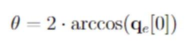
where $\vec{q_{e}}[0]$ is the first entry in the vector $\vec{q_e}$. Similarly, the change of angle error is calculated via

$\dot{\theta_{k}} = \frac{\theta_{k} - \theta_{k-1}}{\Delta T}$

where $\theta_{k}$ is the angle error at timestep $k$. The boolean decision variable $\delta_{RW}$ is introduced which characterizes whether the reaction wheels (RWs) are turned on at any given timestep. In order to avoid frequent changes in the status of the RWs, they are toggled via a hysteresis. For that, upper and lower boundaries for $\theta$ and $\dot{\theta}$ are required:

• $\theta_{\text{max}}$, $\theta_{\text{min}}$
• $\dot{\theta_{max}}$, $\dot{\theta_{min}}$.

The decision variable $\delta_{RW}$ is set as follows:

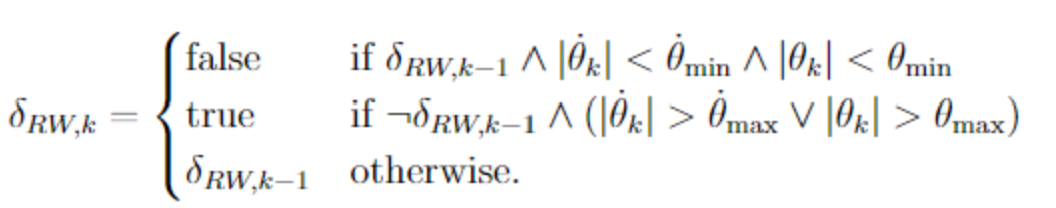
In other words, the RWs are switched off, if the RWs are currently turned on and both $\dot{\theta}$ and $\theta$ are below the lower limit of the hysteresis $\dot{\theta_{min}}$ and $\theta_{min}$. Similarly, the RWs are switched on, if they are currently turned on and either $\dot{\theta}$ and $\theta$ are above the upper limit of the hysteresis $\dot{\theta_{max}}$ and $\theta_{max}$.

Reaction Wheel Desaturation

The reaction wheels can be only spun up to a certain angular velocity. (They have a limited momentum storage.) For us to be able to use them throughout the whole SAGE mission, we need a procedure, called desaturation, to slow them down without applying a net torque on the satellite. To help us with that we have the magnetorquers.

Mathematical explanation

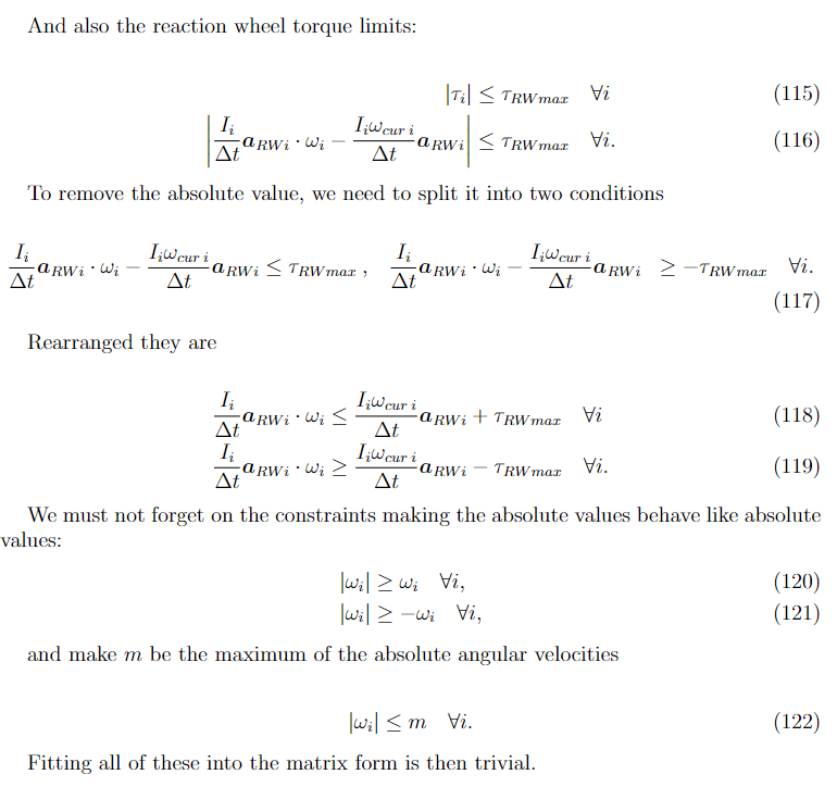
The desaturation problem requires us to find the inputs into the reaction wheels and magnetorquers so that all of the reaction wheel angular velocities are as small as possible at the end, no net torque is applied and all the inputs are within their constraints. Expressed mathematically

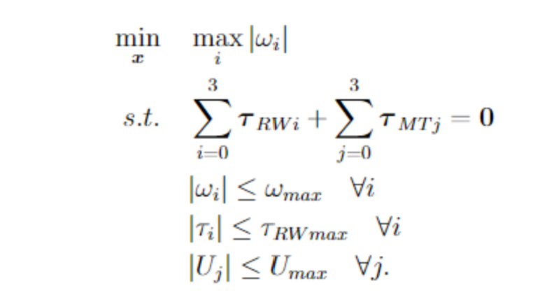
$\omega_i$ is the rotational velocity of the i-th reaction wheel, $\tau_{RWi}$ is the torque applied by the i-th reaction wheel. $\omega_{max}$ and $\tau_{RWmax}$ are the maximum possible velocity and torque of a reaction wheel. $U_j$ is the input voltage into the j-th magnetorquer, $\tau_{MTj}$ is the torque applied by the j-th magnetorquer. $U_{max}$ is the maximum allowed input voltage.

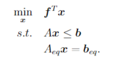
For it to be easily solvable, we need to transform it into a linear program in the standard form:

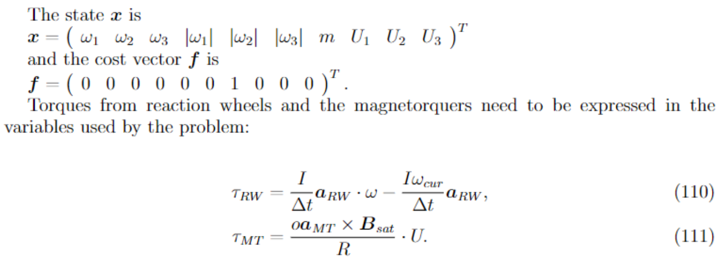
$I$ is the inertia of the reaction wheel around the axis of rotation $a_{RW}$ and $\omega_{cur}$ is its current angular velocity. $o$ is the crossectional area of the magnetorquer, $a_{MT}$ its axis and $R$ its resistance. $B_{sat}$ is the magnetic field of Earth in the satellite coordinate system.

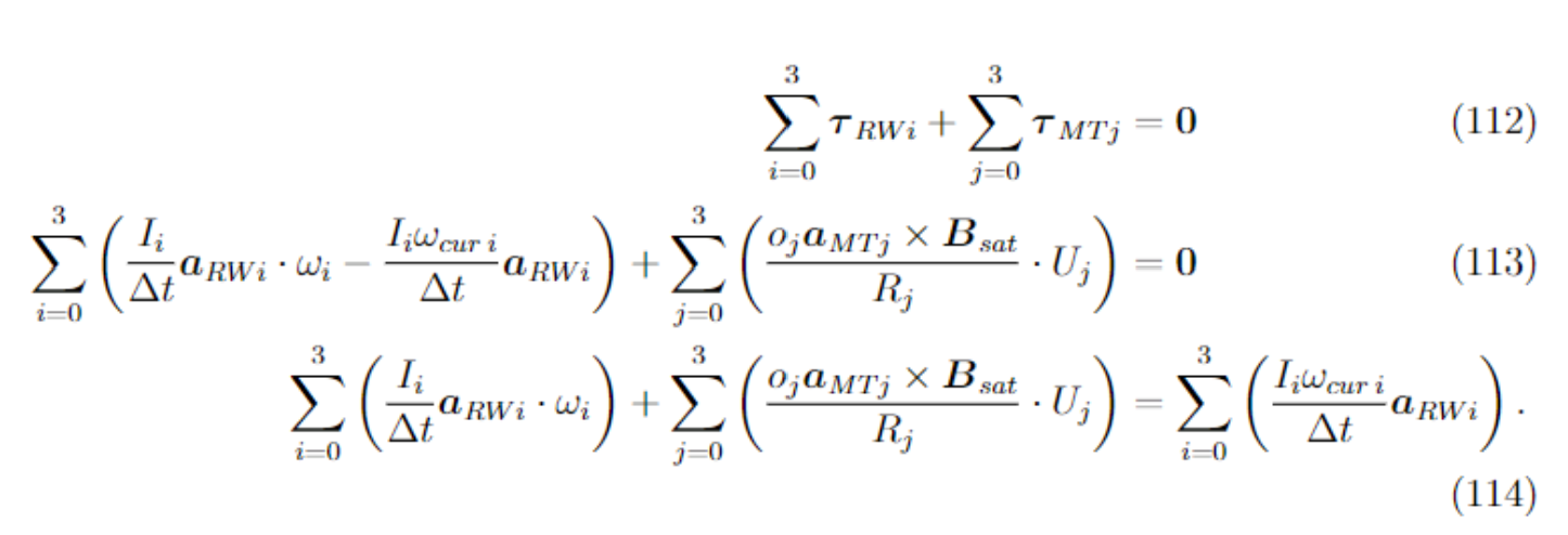
Using these expressions we can rewrite the constraint on the net torque,

CubeSpace

The reaction wheel management designed by CubeSpace is documented on Page 35 in the CubeSpace Commissioning and Operations Manual