Responsible	Samuel Schoenenberger
Last Updated	10/12/2025, 12:48:54 PM
Last Author	Kai Berszin

Satellite Controllers

Scope

This page describes mathematical description and the MATLAB implementation of the Controllers for:

1. Orientation tracking (Sun Pointing and Ground Tracking)
2. Detumbling The controllers designed by CubeSpace are documented on Page 18 to 34 in the CubeSpace Commissioning and Operations Manual

Pointing Controller

The pointing controller allows the satellite to track and maintain a desired attitude.

Mathematical explanation

Functionality

The pointing controller receives the desired attitude $\vec{q}_d$ and the current attitude $\vec{q}_c$ as quaternions.

The pointing error quaternion $\vec{q}_e$ is calculated as the rotation needed to move between the current orientation and the desired orientation $\vec{q}_e = \vec{q}_c^{-1}\cdot\vec{q}_d$

The error rotation quaternion is converted to euler angles pitch (rotation around the x axis), roll (rotation around the y axis) and yaw (rotation around the z axis).

Every angle is fed into its own PID controller that tries to bring the error to 0 independently of other angles.

Performance

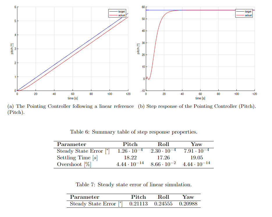
The pointing controller has been tuned and tested for both a step response signal and a linearly increasing reference or target signal.

In the step response experiment, a step of one radian was given as a reference for all three Euler angles. The linearly increasing reference has a slope of 110% of the angular velocity $\omega_{orbit}$ of the satellite at a height $h$ between 450km and 550km above the surface for all three Euler angles. To calculate the orbital speed $v_{orbit}$ the following formula was used: $v_{orbit}=\sqrt{\frac{G \cdot M_E}{R_E+h}}$ $G$ is the gravitational constant, $M_E$ the mass of the earth and $R_E$ is the radius of the earth. Then to calculate the angular velocity this formula was used:

$\omega_{orbit}=\frac{v_{orbit}}{R_E + h}$

This resulted in a $\omega_{orbit}=0.0011 \; rad/s$. Then 110% of $\omega_{orbit}$ was taken as the slope of the linearly changing reference.

The step and linear response properties can be seen in tables 6 and 7. A visualization of the pitch result and target can be found in figures a and b.

Implementation

It is implemented in the file ctrl/pointing/pointingPID.m with the PID tuning parameters:

• $P = (7,7,7)*10^{-5}$
• $I = (1,1,1)*10^{-10}$
• $D = (4,4,4)*10^{-4}$

The controller can be tested with these simulation scenarios (run_files/pointing/):

• run_testPointing.m: linear changing reference tracking
• run_testPointingSinusoidal.m: sinusoidally changing reference tracking
• run_testStatic.m: two static references are matched
• run_trackingAPointingVector.m: Desired orbit frame pointing vector is tracked. This is for sun pointing with the satellite frame vector $(1,1,0)$ and for the ground tracking with the satellite frame vector $(0,0,1)$.

Detumbling Controller

The detumbling controller stabilizes the satellite's angular velocity after separation from the launch vehicle. It is necessary that this stage is as quick and energy-efficient as possible in order to facilitate the start of the research stage of the mission. This section is based on the research and implementation done in Chantal Woodtli's bachelor thesis.

Mathematical explanation

Functionality

After exploring four different types of controllers (standard B-Dot control, orbit dependent B-Dot control, PID-based B-Dot control, Bang Bang B-Dot control), we have chosen to employ a Bang Bang B-Dot controller, since in our simulation it was shown to be the fastest at stabilizing the satellite. The Bang Bang B-Dot controller is based on the B-Dot controller:

$$m_d = -k_b \cdot \dot{b}$$

Where $m_d$ represents the desired magnetic dipole moment on the magnetorquers, $k_b$ is a simple gain and $\dot{b}$ is the temporal derivative of $b$, the magnetic field of the Earth (in the satellite frame of reference).

The Bang Bang approach implements the maximum possible magnetic dipole moment $m_{max}$ at every time frame $k$:

$$m_{k,des} = -m_{max} \cdot sign(b \times \omega_k)$$

Where $\omega_k$ represents the angular velocity vector of the satellite at every time frame $k$. The desired magnetic dipole moment is adjusted in order to avoid saturation of the magnetorquers. The necessary voltage for the magnetorquers to achieve this magnetic dipole moment is extrapolated and directly applied to the magnetorquers.

Performance

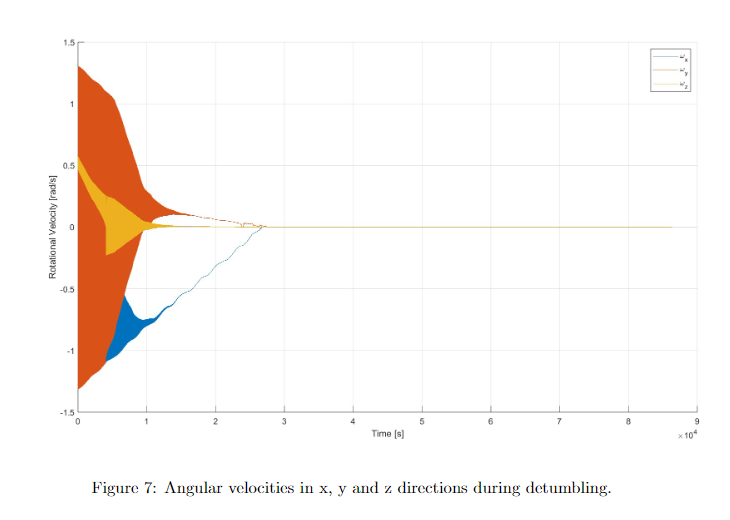
In our simulation the Bang Bang B-Dot controller is able to stabilize the satellite within 7.5 hours. This simulation was performed for the relatively high initial angular velocity of $\omega_0 = (20,30,60)$ deg/s and the calculated disturbance torque. Figure 7 shows the angular velocities of the satellite during the first 24 hours after detachment.

Implementation

The simulation for the detumbling is implemented in run_files/detumbling/run_testDesaturationController.m.

The controller for detumbling is implemented in ctrl/detumbling/bDotBangBang.m.