Responsible	Samuel Schoenenberger
Last Updated	10/12/2025, 12:48:54 PM
Last Author	Kai Berszin

Estimators

Scope

This article describes the state estimation requirements and the Extended Kalman Filter designed for state estimation.

State Estimation Requirements

Internal state of the satellite for the purposes of attitude determination includes:

1. 3 DoF Orientation
2. Angular velocities Additional information needed:
3. Earth's magnetic field at the current location
4. The Sun's position relative to the current location This information is provided by the MOPS team in a form of a lookup table based on the current time, which can be obtained through the GNSS antennas. Using the sensors specified earlier we can use the full state EKF documented at Page 13 to 17 in the CubeSpace Commissioning and Operations Manual

Extended Kalman Filter

Accurate estimation of the CubeSat's state, including attitude $\vec{q}_O^B$ and angular velocity $\vec{\omega}_O^B$, is crucial for proper navigation and control. Gyroscope, accelerometer and magnetometer readings are therefore combined into a Dual Kalman Filter to achieve an attitude estimation accuracy of below $3^{\circ}$ defined by the communication constraints.

Angular Velocity

Mathematical explanation

The angular velocity estimation is based on this paper using gyroscope and accelerometer readings as the observed measurements. The estimation is further complemented by the sensor biases for each sensor on each axis individually, resulting in the following state vector:

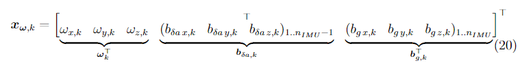
Where $n_{IMU}$ is the number of available IMU's. The accelerometer biases consist of one triple less, as the differences between accelerometer readings are considered to be the measurements

Measurement model

The acceleration measured by an accelerometer $\vec{a_i}$ at position $\vec{r_i}$ in body frame is described by

$\vec{a_i} = \vec{a} + \vec{\omega} \times (\vec{\omega} \times \vec{r_i}) - \vec{r_i}\times\vec{\dot{\omega}} +\vec{n_{a_i}}$

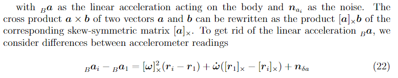
Which can be rewritten as

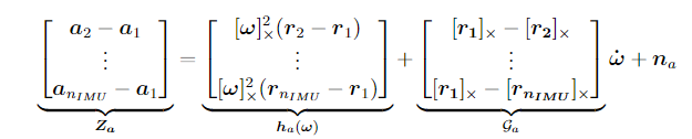
where $\vec{n_a}$ is the noise with covariance matrix $\mathcal{R_a} = 2\sigma_a^2 \mathcal{I_{3(n_{IMU}-1)}}$ with $\mathcal{I_{3(n_{IMU}-1)}}$ as the identity matrix of size $3(n_{IMU}-1)$.

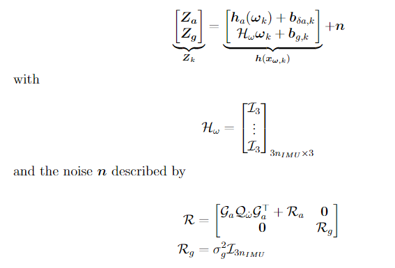
As the angular acceleration $\vec{\dot{\omega}}$ is unknown, it's considered an additional noise term in the form of $\mathcal{G_a} \mathcal{Q_{\dot{\omega}}}\mathcal{G_a^T}$ with $\mathcal{Q_{\dot{\omega}}} = \sigma_{\dot{\omega}}^2\mathcal{I_3}$. Combined with the gyroscope measurements $\vec{Z_g}$, the measurement equation is given by

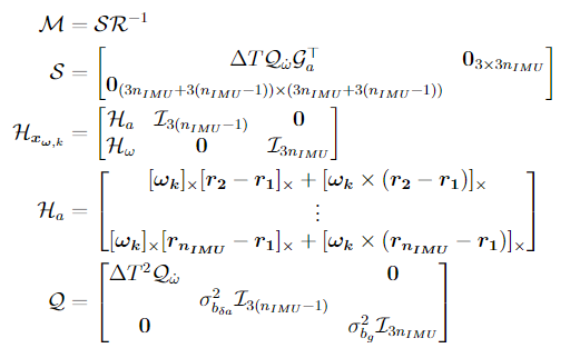
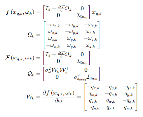
Prediction

The prediction of the current state $\vec{x_{\vec{\omega},k}^{pred}}$ and covariance $\mathcal{P_{\vec{\omega},k}^{pred}}$ based on the previously estimated state $\vec{x_{\vec{\omega},k-1}^{estim}}$ and covariance $\mathcal{P_{\vec{\omega},k-1}^{estim}}$ is done using:

with

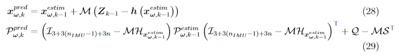
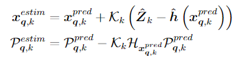
Estimation

The estimation of the current state $\vec{x_{\vec{\omega},k}^{estim}}$ and covariance $\mathcal{P_{\vec{\omega},k}^{estim}}$ based on the predicted state $\vec{x_{\vec{\omega},k}^{pred}}$ and covariance $\mathcal{P_{\vec{\omega},k}^{pred}}$ is done using:

with

Implementation

The simulation can be found in run_files/attitude_estimation/run_angular_velocity_EKF.m and the implementation at angularVelocityEKF.m.

Attitude (Orientation)

Mathematical explanation

The estimated angular velocity $\vec{\omega_{k}^{estim}}$ is then used as the control input for the attitude estimation based on this source with only magnetometer readings as the measured input. The bias estimation for the magnetometers has been added here as well:

Where $n_{m}$ is the number of available magnetometers.

Measurement model

The magnetometer measurement $\vec{m}_i$ can be described as follows $\vec{m_i} = \mathcal{R}(\vec{q})\vec{h_m}$

where $\mathcal{R}(\vec{q})$ rotates the expected magnetic measurement $\vec{h_m}$ from the Earth frame to sensor frame around the attitude $\vec{q}$. This can be rewritten as

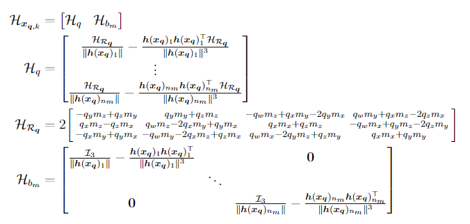
where the noise $\vec{n}$ is described by $\mathcal{R} = \sigma_m^2\mathcal{I_{3n_{m}}}$ To be comparable, $\vec{Z_k}$ and $\vec{h}(\vec{x_{\vec{q},k}})$ have to be normalized

This results in following Jacobian $\mathcal{H_{\vec{x_{\vec{q},k}}}}$ for the measurement model:

Prediction

he prediction of the current state $\vec{x_{\vec{q},k}^{pred}}$ and covariance $\mathcal{P_{\vec{q},k}^{pred}}$ based on the previously estimated state $\vec{x_{\vec{q},k-1}^{estim}}$ and covariance $\mathcal{P_{\vec{q},k-1}^{estim}}$ is done using:

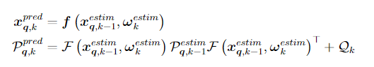
with

Estimation

The estimation of the current state $\vec{x_{\vec{q},k}^{estim}}$ and covariance $\mathcal{P_{\vec{q},k}^{estim}}$ based on the predicted state $\vec{x_{\vec{q},k}^{pred}}$ and covariance $\mathcal{P_{\vec{q},k}^{pred}}$ is done using:

with

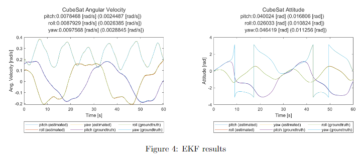
Results

The EKF successfully stays within the $3^{\circ} \approx 0.052 rad$ on noisy measurements and fast changing state.

Implementation

The simulation can be found in run_files/attitude_estimation/run_ekf.m and the implementation of the math at state_estimation/ekf/EKF.m.

Sensor Fault detection

Mathematical explanation

The State estimation pipeline must be resilient to faults in the sensor that could propagate inside the Extended Kalman Filter and make the current estimated state not reliable. For this, we implemented an approach based on this paper using the Innovation covariance. Detecting a large increase in these coefficients signifies that the estimated state is inconsistent with the measurements. The Innovation covariance is calculated as: $\mathcal{V_i} = (\vec{z_i} - \vec{y_i})(\vec{z_i} - \vec{y_i})^T$ where $z_i$ is the measurement of the state vector at timestep $i$ and $y_i$ is the estimate of the state vector at timestep $i$. We calculate the moving average of these matrices over $N$ timesteps:

$\mathcal{V_{i}^{*}} = \frac{1}{N} \sum_{k=i-N}^{i} \mathcal{V_i}$

The values we need to monitor are the diagonal values:

$\vec{J_i} = diag(\mathcal{V_{i}^{*}})$

To detect large changes in the elements of $\vec{J_i}$, we use the CUSUM algorithm taken from here. During simulation, the means and standard deviations of these coefficients are first learned, then one of three types of faults is added: large additive constant, signal replaced by white noise, and ramp.

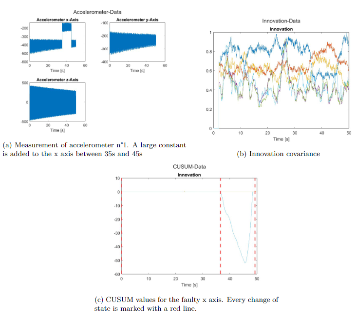
The means and standard deviations of $\vec{J_i}$ are learned over 10 seconds, the moving average window size $N$ is 0.2s. The fault is detected at 35.96s and ends at 47.47s.

Sun Detection

This chapter describes how we could use the sun sensors to detect the direction to the Sun.
To accurately calculate a sun vector coming from any direction, full sky coverage is required. This means that a sun sensor would be required on each of the six sides of the CubeSat. So for the majority of cases it is not possible to have three overlapping sun sensor field of views, we will be calculating 2 possible candidates that could be the correct sun sensor with the information from 2 sun sensors with overlapping field of views.
If a third sensor happens to have an overlapping field of view, the angle between the surface normal of the surface with the third sensor will be checked to choose one of the sun sensor candidates.

Mathematical explanation

This example is done with the sun sensor at the center of the +x and the +y surfaces.
To calculate a vector it is important to have 2 points. The sun vector will be at the overlap border of the two cones created by the angles $\theta_1$ and $\theta_2$. The first point, let's call it $P$, is where the cones meet on the xz-plane. Additional known parameters are the half lengths of the satellite surfaces $d_1$ and $d_2$ It is visualized in Figure 1.

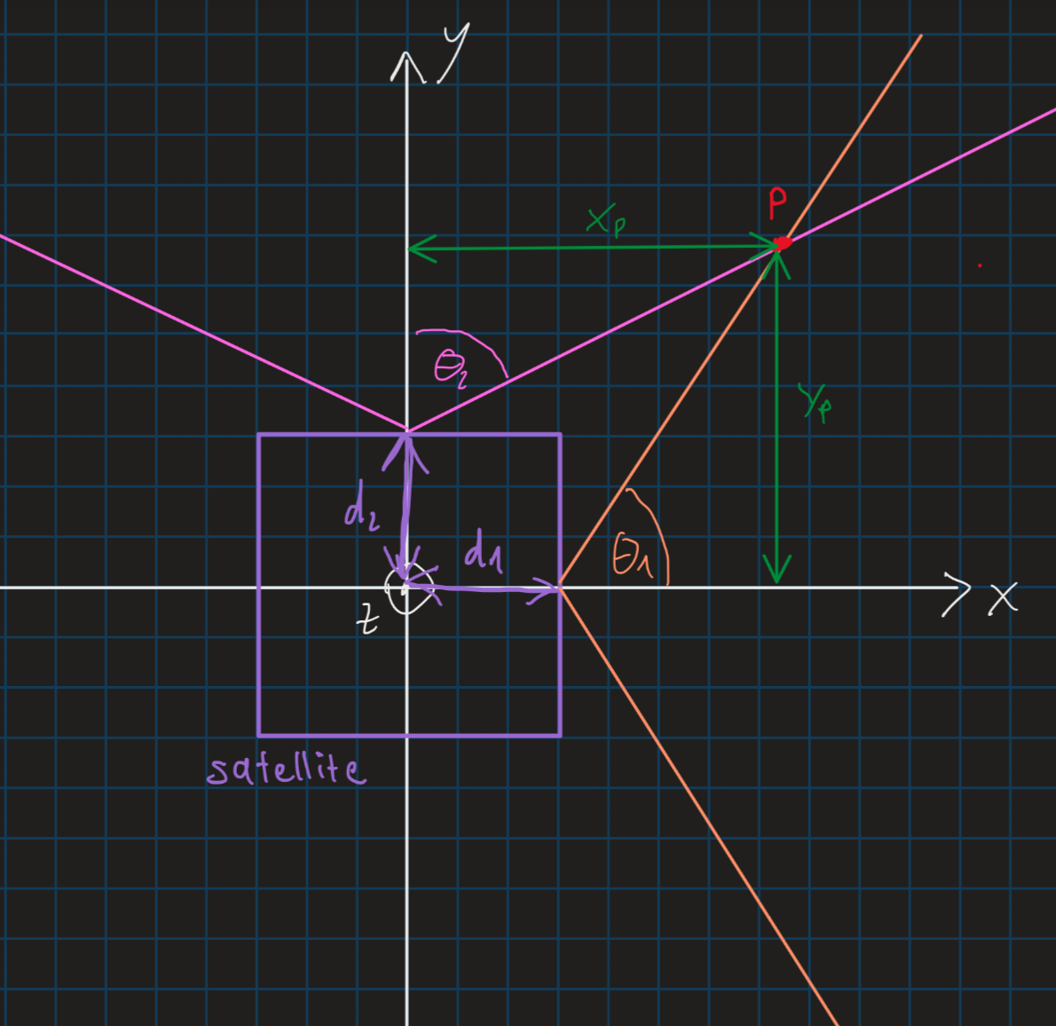
From Figure 1 we can derive the formulas: $\tan\theta_1 = \frac{y_p}{x_p - d_1}$ $\tan\theta_2 = \frac{x_p}{y_p - d_2}$ from which we derive $x_p = \frac{\tan\theta_2 (\tan\theta_1 \cdot d_1 + d_2)}{\tan\theta_1\cdot\tan\theta_2 + 1}$ $y_p = \frac{\tan\theta_1 (\tan\theta_2 \cdot d_2 + d_1)}{\tan\theta_1\cdot\tan\theta_2 + 1}$ so we get $P=(x_p,y_p,0)$ For the second point to calculate a vector needs to be in the overlap area of the sun sensor field of views. But since we lack a degree of freedom to definetely know the point so two candidate points $Q_1$ and $Q_2$ are considered. $Q'$ is the projection of both points onto the xy-plane. Since it needs to be in the overlap area so we fix $x_q = x_p + 1$. From there we calculate $y_q$, $z_{q}$ and $z_{p}$.

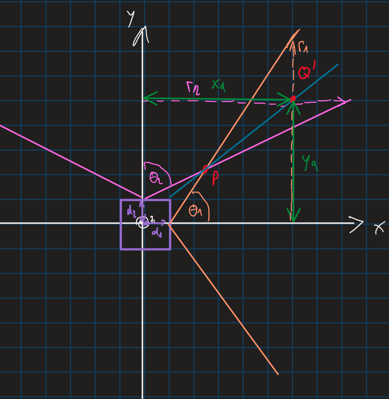
From Figure 2 we can derive the formula $\tan\theta_1 = \frac{r_1}{x_q - d_1}$ and $\tan\theta_2 = \frac{r_2}{y_q - d_2}$

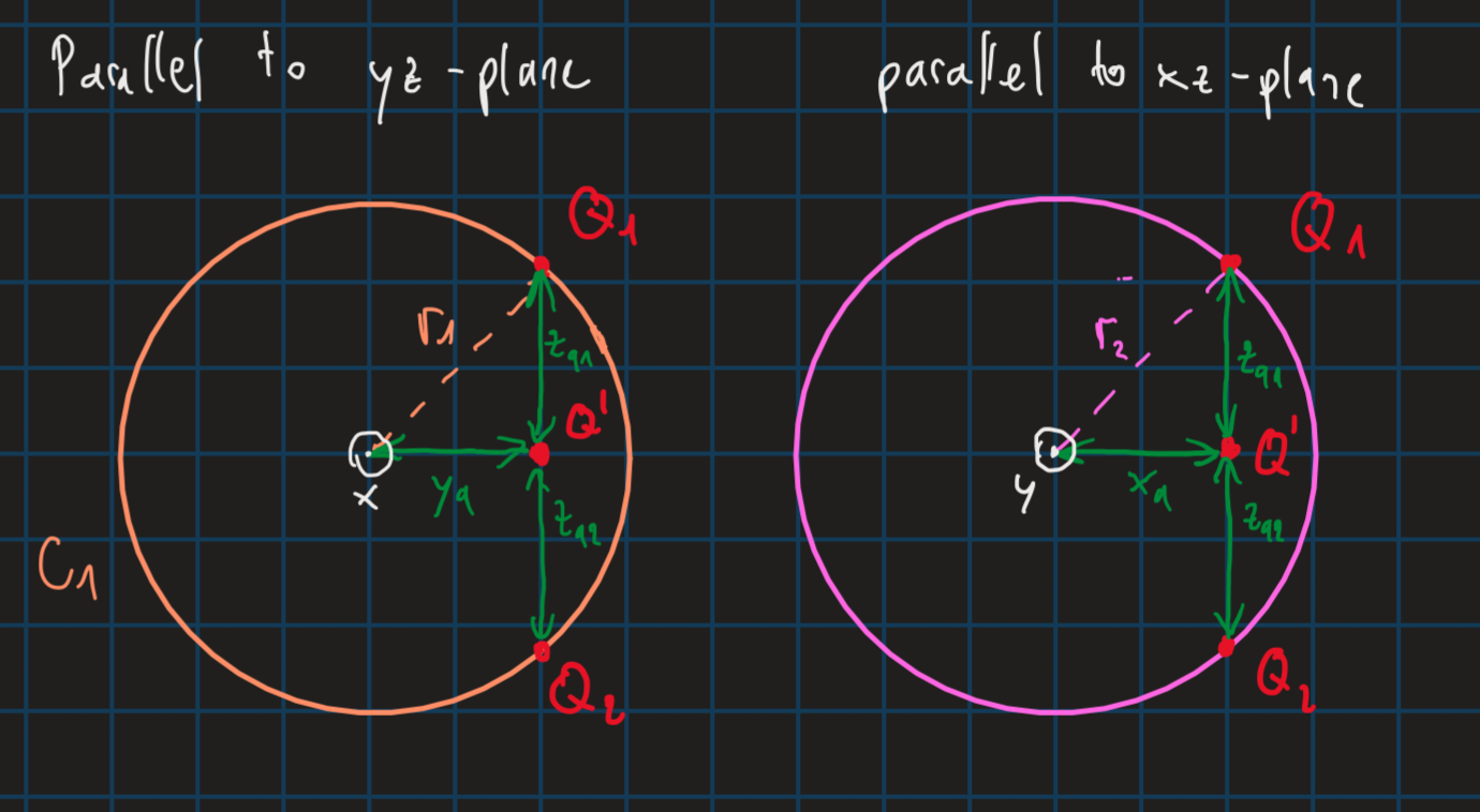
And from Figure 3 we can observe: $z_{q}^2=z_{p}^2=r_2^2-x_q^2$ and $y_q^2=r_1^2-x_q^2$ Solving these for $y_q$ and $z_q$ we get $y_q = \sqrt{\frac{1+\tan^2\theta_1}{1+\tan^2\theta_2}x_q^2}$ and $z_{q}=\sqrt{\frac{1+\tan^2\theta_1}{1+\tan^2\theta_2} \tan^2\theta_2 - 1}x_q$ and we also know that $z_{p}=-z_{q}$.
Finally, we have the points $Q_1 = (x_q,y_q,z_{q})$ and $Q_2 = (x_q,y_q,z_{p})$. From here we get the sun sensor candidates $v_{SV1}$ and $v_{SV2}$ with the following formulas: $v_{SV1}=\frac{P-Q_1}{\parallel P-Q_1 \parallel}$ and $v_{SV2}=\frac{P-Q_2}{\parallel P-Q_2 \parallel}$

Implementation

The simulation is implemented in run_files/sun_detection/run_testSunDetection.m. It is implemented in an if-else check structure that checks whether any viable combination of sun sensor angles have been read out by the coarse sun sensor object. This is implemented in the file state_estimation/sun_detection/detectSun.m. If only 2 sun sensors detect the sun, both sun sensor candidate vectors are returned. The actual calculation of the two sun sensor candidates happens in the file state_estimation/sun_detection/calculateSunVectorWith2CoarseSunSensors.m.
The inputs are the angles $\theta_1$ and $\theta_2$ and the surface normals of the surface that the sun sensor is located on. The $d_1$ and $d_2$ parameters are based on the surface of choice. The function is implemented so that this algorithm works with any combination of neighbouring surfaces.

If 3 sun sensors detect the sun only one sun sensor candidate is returned. This check function is implemented in state_estimation/sun_detection/calculateSunVectorWith3CoarseSunSensors.m. This check function calculates the angle between the surface normal of the +z axis and the two sun vector candidates. The one that has an angle that is within the field of view of the sun sensor is chosen as the final sun vector and returned.

Additionally, if only one sensor detects the sun but with an angle smaller than 3 degrees, it returns the surface normal of the sun senosr's corresponding surface as the sun vector.

The getDummySunVector.m returns a simulation scenario of a reference sun vector based on a seed for the simulation.

Magnetic Field Estimation

Mathematical Explanation

The earth's magnetic field can be determined with the measurements of the magnetometers. As the sensors have biases, they have to be subtracted from the measured values to get the actual measurement. The estimate of the magnetic field can then be determined with a weighted least square algorithm as follows: $\vec{x}=(\mathcal{H}^T\mathcal{R}^{-1}\mathcal{H})^{-1}\mathcal{H}^T\mathcal{R}^{-1}\vec{z}$ with x being the magnetic field estimate and z the measurements represented as a vector. The matrix H represents the rotation between the magnetometer and the satellite frame. The matrix R is the covariance matrix of the measurements which is used to weight the measurements. The bigger the variance the less the value is weighted for the estimation.

Implementation

The simulation is implemented in run_files/magnetic_field_estimation/run_magneticEstimation.m and algorithm is implemented in state_estimation/magnetic_field_estimation/estimate_magnetic_field.m.