Responsible	Samuel Schoenenberger
Last Updated	10/12/2025, 12:48:54 PM
Last Author	Kai Berszin

Simulation Setup

Scope

Includes mathematical description as well as description of MATLAB implementation of satellite coordinate frames, satellite dynamics and disturbance torques.

Coordinate Frames

For our calculations, we use three different coordinate frames:

Earth Frame (E)

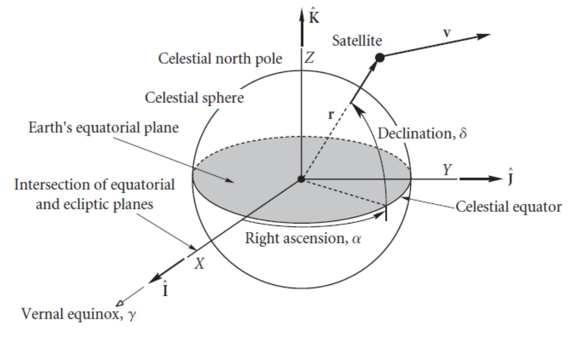
The Earth frame E has its origin at the center of mass of the Earth. The z-axis (z_E) is aligned with the Earth's rotation axis, and the x-axis (x_E) is aligned with the mean vernal equinox. The vernal equinox is the intersection of the equatorial and ecliptic planes. The Earth's equatorial plane is the plane passing through the equator of the Earth. The Earth's ecliptic plane is defined as the imaginary plane containing the Earth's orbit around the sun. The y-axis (y_E) completes the right-hand set of coordinate axes.

Orbit Frame (O)

The orbit frame O has the exact same orientation as the Earth frame E, but its origin is located at the geometrical center of the satellite. The three axis are x_O, y_O and z_O respectively.

Satellite Body Frame (B)

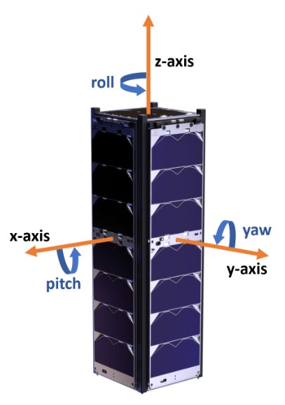
The satellite body frame B also has its origin at the geometrical center of the satellite. The z-axis is parallel to the structure rails, and the UHF and S-band antenna should be located on the -z end. The three axis are x_B, y_B and z_B respectively.

Satellite Dynamics

Mathematical Description

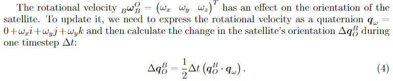
The satellite state has two components. The rotation quaternion $\vec{q}_O^B$ representing the rotation from the orbit frame to the satellite body frame. And the rotational velocity of the satellite body frame with respect to the orbit frame, represented in the satellite body frame $\vec{\omega}_B^O$. The dynamics of the satellite were derived in a Bachelor's thesis by Carolyn de Oliviera Baumann and Fabienne Maissen.

The rotational dynamics are:

Where $\mathcal{I} \in \mathbb{R}^{3\times 3}$ is the inertia matrix of the satellite and $\vec{\omega}_B^O \in \mathbb{R}^{3}$ its angular velocity. The torque on the satellite $\vec{\tau} \in \mathbb{R}^{3}$ consists of two parts, the torque exerted by the actuators $\vec{\tau}_a$ and the disturbance torque $\vec{\tau}_d$: $\vec{\tau} = \vec{\tau}_a + \vec{\tau}_d$

The translation dynamics are not important for the design of the attitude determination and control system.

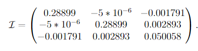
In our simulations we used the inertia matrix calculated by the structures team:

Implementation

To verify our controllers, this model was implemented as a MATLAB simulator with numerical integration of the differential equations done using the Runge Kutta method of the 4th order. It is implemented in the simulation/Satellite.m file in the sim_rungekutta function.

Disturbance Torque

Mathematical Description

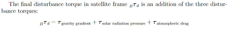
There are three sources of the disturbance torque $\vec{\tau}_d$: Gravity Gradient, Solar Radiation Pressure and Atmospheric Drag.

The gravity gradient is caused by Earth's gravity and aligns the satellite's longitudinal axis towards the center of the earth. The torque's strength depends on the orbital radius.

The radiation from the Sun enacts a force and thus a torque onto the satellite, which has to be taken into account. While the atmosphere in LEO is thinner than on the ground, it is not a vacuum, meaning that aerodynamic forces influence the satellite.

Implementation

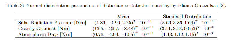
Each disturbance is modelled by a Gaussian distribution with a mean and standard deviation that has been calculated based on simulation that was performed by Blanca Crazzolara. It is implemented in simulation/getDisturbanceTorques.m.

Hardware Models

Reaction Wheels

The Reaction wheel is implemented as a class in simulation/actuators/ReactionWheel.m. The Array of reaction wheels is implemented in simulation/actuators/RWarray.m. The reaction wheels are implemented with the following hardware parameters taken from the documentation of the CubeWheel CW0017 from CubeSpace. The reaction wheel array class is initialized for the simulation with these parameters in auxiliary/setupParams.m.

Magnetorquer

The Magnetorquer is implemented as a class in simulation/actuators/Magnetorquer.m. The Array of all magnetorquers put together is implemented in simulation/actuators/MTarray.m. The Magnetorqers are implemented with the following hardware parameters taken from the documentation for the CubeTorquer CR0003 from Cube Space in the auxiliary/setupParams.m file, where the entire array of magnetorquers is initialized.

Magnetometer

The array of the magnetometer is implemented in simulation/sensors/MagnetometerArray.m and the individual IMU is defined as a class in simulation/sensors/Magnetometer.m. For the simulation it is initialized in the setupParams.m file. They are not currently implemented with Cube-parameters.

Fine Sun Sensor

The fine sun sensor is not currently implemented in the simulation.

Coarse Sun Sensor

The coarse sun sensor is implemented as a class in simulation/sensors/coarseSunSensors. m.

Earth Horizon Sensor

The earth horizon sensor is not currently implemented in the simulation.

IMU (Inertial Measurement Unit)

The array of the IMU's is implemented in simulation/sensors/IMUarray.m and the individual IMU is defined as a class in simulation/sensors/IMU.m. The parameters are implemented in the setupParams.m. They are not currently implemented with Cube-parameters.

Reference Calculators

The reference calculators convert external commands and data to references the controllers should track. Functions:

1. Ground station tracker
2. Sun tracker